[Apologies, I initially published two posts out of order.]
I’m working on turning my blog into a book, and in order to do that I need to give readers an idea of how I ended up where I am today. One obvious need is to explain how I adopted a quantity theoretic approach to monetary analysis, rather than some alternative like the interest rate approach. For me it all goes back to the Great Inflation of the 1960s to the early 1980s.
As an aside, the quantity theory can be defined in several ways:
1. An X% rise in M will be associated with an X% rise in P
2. An X% rise in M will be associated with an X% rise in NGDP
3. An X% rise in M will cause both P and NGDP to be X% higher than otherwise, in the long run.
The third definition is probably the most accurate, and the first is the least accurate.
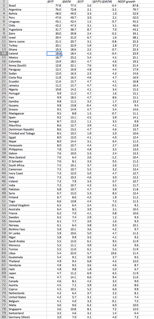
The following data set (from a Macroeconomics textbook by Robert Barro) is so rich in information, that we will spend many posts investigating all the implications. It shows average inflation, money growth and real GDP growth rates over 30 or 40-year periods around 1950-90, for 79 countries:
Right off the bat one notices the strong correlation between the growth rate of M (the monetary base) and P (the price level.) David Hume didn’t have this data set in 1752, but just using his brilliant mind he was able to figure out that if you double the money supply, the only long run effect is for prices to double. Money is just a measuring stick. For about 40 years Argentina and Brazil were doubling the money supply, on average, once every 14 months. And prices were doubling just as Hume predicted. All good, the Quantity Theory of Money (QTM) is triumphant.
Except it’s all downhill from here. I’ve just provided the best possible data set for convincing you of the QTM. Suppose I had only given you the bottom half of the data set? Now the correlation is much harder to see. Or suppose we’d looked at shorter time periods. Again, not so good. Or suppose we’d looked at countries at the zero bound? Now the QTM would have major problems.
The key to understanding the QTM is to hold two thoughts in your mind at the same time. In one sense the theory is logical, indeed blindingly obvious. It’s incredibly powerful, incredibly true. But in all sorts of situations it seems to fail. That’s what we need to figure out.
Before moving on, let’s remind ourselves why it’s the bedrock of monetary theory, and why all other theories fall short. In this data set we are doing the economic equivalent of when scientists expose objects to great heat, pressure, or speed, to get at the essential qualities. We’re looking at what happens with very fast money growth
No other model can explain the correlations we see. Yes, the growth in the money supply might have “root causes” elsewhere, such as budget deficits. But you can’t figure out that Brazil and Argentina would have 75% inflation for 40 years, whereas Iceland would have 19% and the US would have 4% by looking at budget deficits, you need the money supply growth rates to even get in the right ballpark. Note that some countries (the US in the 1970s) printed lots of money w/o big budget deficits.
Nor do interest rate models work. Ironically the only interest rate model that would even come close is NeoFisherism, as the nominal interest rates in these countries would also be highly correlated with inflation. But that model doesn’t tell you how you get those high nominal interest rates. Again, you need money supply data.
Nor will an exchange rate model work. Yes, the (depreciating) exchange rate for Brazil and Argentina was closely paralleling their inflation rate. They saw the local currency price of US dollars rise at around 70% per year over those 40 years. But that doesn’t explain how you cause the currency to depreciate so rapidly over 40 years. Again, you need money supply data. Both the Fisher effect and PPP are just appendages of the QTM.
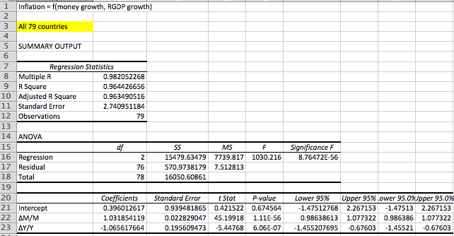
Let’s finish today’s post with the first of several regressions that I’m going to give you–all provided by Patrick Horan of the Mercatus Center:
 This is the Mona Lisa of macro regressions. The t-statistic on money growth is 45.2. Yup, I’d say there’s some truth to the QTM. The P-value? One over . . . umm . . . how many atoms are there in the universe? And the coefficient is pretty close to one, within two standard errors. When you raise the money supply at 75%/year for 40 years, you’ll get roughly 75% inflation.
Later we’ll see there’s a reason the coefficient is slightly greater than one. Can you guess? (It’s a very hard question.) But let’s finish up by noticing the coefficient on real GDP growth (delta Y). You’ve all been taught that economic growth is inflationary. The people at the Fed tell us that inflation will rise as we approach full employment. Maybe it will, but not because growth is inflationary. As you can see from the regression, economic growth is deflationary, indeed almost exactly as deflationary as money growth is inflationary. So are the Keynesians wrong?
Yes they are! And they are wrong in an interesting way. Let’s suppose their predictions turn out right, and inflation does rise as we approached full employment. Will I admit that I’m wrong? Of course not!! I’m an arrogant economic blogger. Instead I’ll claim that this bizarre outcome is proof of the Fed’s incompetence. They so botched monetary policy that they made inflation procyclical. Indeed they do this so often that some of my commenters think this is natural. Poor Mr. Ray Lopez found a dictionary somewhere that says inflation naturally falls during recessions and rises during booms.
And it’s all a myth. Don’t worry, we’ll explain the mystery of deflationary growth in the next post. And we’ll explain why the coefficient on money growth was a little bit bigger than one in the post after that. All our money/macro questions are answered in this data set, if we know where to look. Put on your David Hume thinking hat, you have lots more info to work with than he had. Indeed Milton Friedman became the second most famous economist of the 20th century mostly by figuring out how this data set allowed us to go “one derivative beyond Hume.”
PS. Here are the two “money quotes” (pun intended) from Friedman:
Double-digit inflation and double-digit interest rates, not the elegance of theoretical reasoning or the overwhelming persuasiveness of serried masses of statistics massaged through modern computers, explain the rediscovery of money.” (1975, p. 176.)
As I see it, we have advanced beyond Hume in two respects only; first, we now have a more secure grasp of the quantitative magnitudes involved; second, we have gone one derivative beyond Hume.” Friedman (1975, p. 177.)
