Black & Scholes for Puts/Calls in a Single Excel Cell

Sometimes an online option calculator isn’t enough and you’d like to implement the Black & Scholes (B&S) option pricing equations in Excel.  If you’re just playing around it doesn’t matter how you structure the calculation.  In fact, for clarity’s sake, it’s probably a good idea to spread out the calculation across multiple cells.  However, if you’re planning to do some serious work with multiple B&S calculations then having the formula condensed into one cell is very useful.  For example, it enables a simple copy and paste operation to create a two-dimensional array of option price calculations.

This post describes a parameterized single-cell B&S
calculation that handles either put or call options and shows how it can be
used as a building block for several different types of option
simulations.  At the end there’s a procedure
for downloading a free copy of the spreadsheet containing the single-cell
formula and several example usages.  For
a nice tutorial treatment of the B&S equations in Excel see this
MacroOption post.
 

The Equations

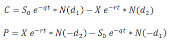
The Black & Scholes Option Price Equations, including
dividends for calls (C) and puts (P) are:

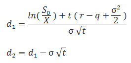
Where:

The parameters / symbols / abbreviations are:

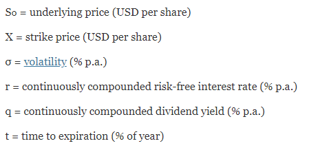
Elaborations:

• (% p. a.) = Annualized percentage
•  e^x  = Euler’s number to the X^th power,
  implemented as exp() in Excel
• ln(x) = Natural Logarithm of x, implemented as
  ln(x) in Excel
•  N(x)  = Cumulative Standard normal distribution,
  with mean of zero and standard deviation of one, implemented as Norm.S.Dist
  (x,1) in Excel

An Excel Implementation

• The put and call versions of the Black &
  Scholes equation are shown as separate equations above but the two equations
  can be merged into a single equation by adding an additional parameter which
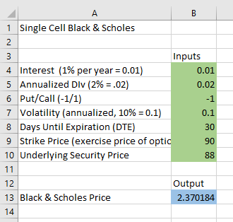
  has the value of 1 for calls and -1 for puts.
• In the worksheet “Single” of the Excel
  spreadsheet I created, I use absolute cell references (e.g., $B$5) for all 7
  parameters. Using absolute cell references simplifies making more complex
  arrangements later.
  • $B$4: 
    Interest Rate (1% per year = 0.01)
  • $B$5: 
    Annualized Dividend Rate (2% per year = 0.02)
  • $B$6: Put/Call Switch (Put = -1, Call = 1)
  • $B$7: Annualized Volatility (10% = 0.1)
  • $B$8: Days until Expiration
  • $B$9 Strike Price (exercise price of the option)
  • $B$10 Underlying Security Price
• The B&S pricing formula in the Single sheet
  • =$B$6*$B$10*EXP(-$B$5*$B$8/365)*NORM.S.DIST($B$6*(LN($B$10/$B$9)+($B$4-$B$5+$B$7^2/2)*$B$8/365)/($B$7*SQRT($B$8/365)),1)-$B$6*$B$9*EXP(-$B$4*$B$8/365)*NORM.S.DIST($B$6*((LN($B$10/$B$9)+($B$4-$B$5+$B$7^2/2)*$B$8/365)/($B$7*SQRT($B$8/365))-$B$7*SQRT($B$8/365)),1)
• The Single worksheet of the spreadsheet looks like this:

Modeling Option Prices with the Black & Scholes
Equations

To show how this single cell implementation of the B&S can be useful, I’ll go through a detailed example copying this single sheet and then modifying it to set up a two-dimensional simulation of option prices, varying both the value of the underlying and the time until expiration. 

Steps

1. Copy & paste the entirety of the “Single”
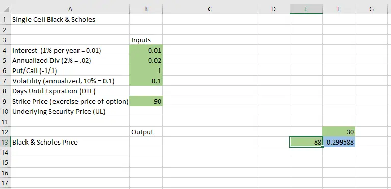
   sheet to another sheet, my example sheet is “2D example”
2. On the new sheet, drag (or Cut and paste)
   the B&S equation cell from B13 to F13. 
   Since all the parameters use absolute references (e.g., $B$5) the
   parameters all stay the same.
3. Drag (or Cut & paste) the Days Until
   Expiration cell (DTE), $B$8 to F12.  When
   you do this operation Excel will change the Days until Expiration references in
   the equation from $B$8 to $F$12.  It is
   important to do cut & paste, not copy & paste because Excel will not
   modify the formula if you just do a copy operation.
4. Drag (or Cut & paste) the Underlying
   cell $B$10 to Days to E13. 

The spreadsheet now looks like this:

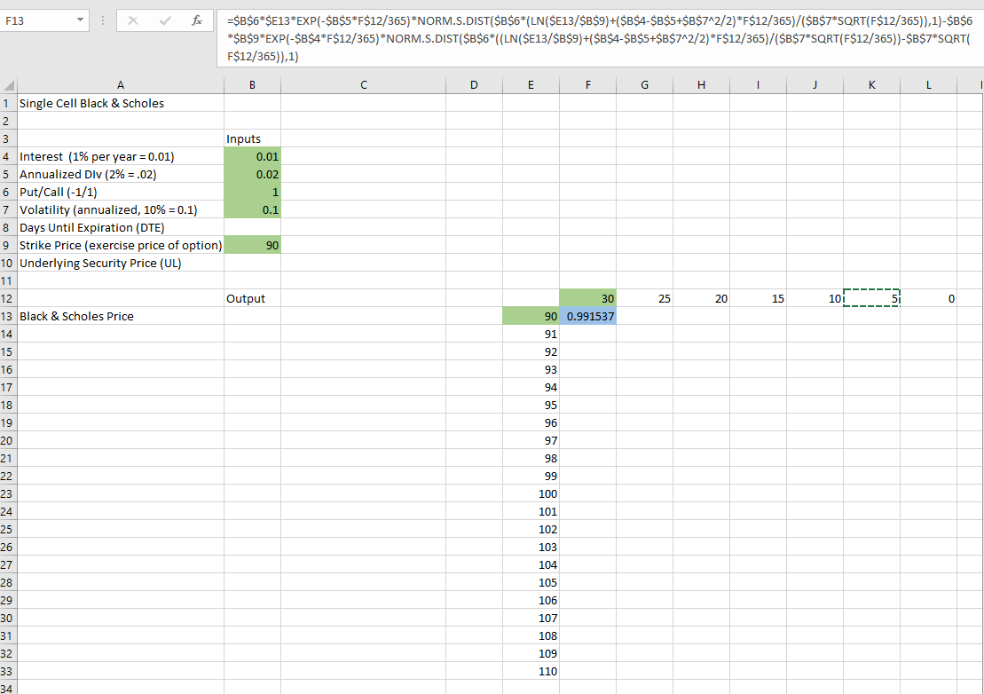
• Now I create the range of the Underlying (UL)
  and DTE values that I want to use.  I
  type ‘=D13+1’ in cell E14 (no quotes) and then copy cell E14 from E15 to E33,
  and I type ‘=F12-5’ into G12 and then copy G12 into Cells H12 through L12.
• Next, I want to change the UL and DTE references
  in the formula from absolute cell references to be relatively referenced.  This allows the formula to access variables
  placed in the appropriate rows and columns respectively.  To do this I use Excel’s find and replace
  function to exchange all UL references, $E$13 in the formula with $E13 and all
  DTE references, $F$13 with F$13. These references are used a total of 10 times
  in the formula.  Doing these changes manually
  even once is error-prone. The sheet now looks like this.

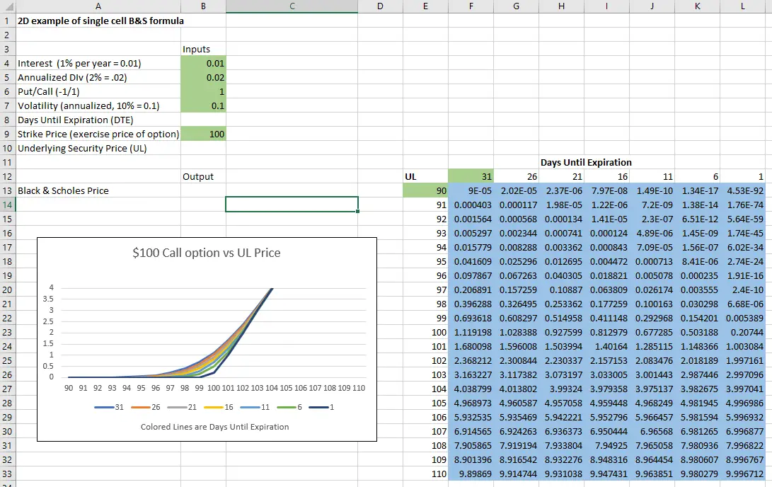
Now, after those changes, I can copy & paste the B&S
formula in F13 into F13 though L33 and Excel will automatically change the cell
references for UL and DTE to reference the appropriate cells.  After doing this copy & paste, changing
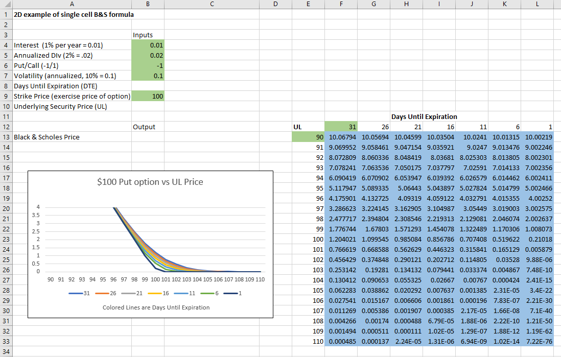
the Strike price to $100 in cell b9, changing the Days to Expiration to 31 in
F12, and doing a little formatting/charting, I have the following result.

Changing the Call/Put parameter B6 from 1 to -1 gives the put dynamics:

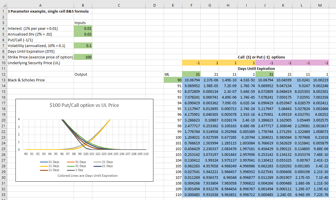
Any of the B&S parameters can be made into a variable using
the approach I demonstrated above.  The
next picture shows the Put/Call parameter turned into a variable also.  The sheet is named “Puts + Calls”.

Modeling Issues

Probably the biggest weakness of the B&S model is that
it assumes that options will exhibit the same implied volatility regardless of
what strike they are at, or how long they have until expiration.  The market knows this is a bad
assumption.  For example,
out-of-the-money (OTM) puts will tend to have a higher price than the B&S
approach would predict.

You can compensate for implied volatility dynamics in simulations
by making the volatility parameter, a computed variable (e.g., you could make
volatility dependent on the difference between the underlying and the strike
price).  Unfortunately, it’s challenging
to model implied volatility reliably. 
For example, if the market does have a correction sometimes the implied
volatility of an OTM put stays the same even when the underlying price has
dropped considerably.

The good news is that unless you’re trying to do some pretty
sophisticated modeling a constant volatility assumption is probably good
enough.

Conclusion

Developing an investment strategy that uses options is a
difficult exercise.  Options strategies require
selection of strike prices, expiration dates, and roll procedures.  Once developed it’s tough to backtest strategies
that include options because historical options data is seldom free, usually
has errors, and often lacks important information (e.g., Greeks).

While far from a perfect tool, using the Black & Scholes equation for simulating option strategies is relatively straightforward, requiring estimates of only three parameters, implied volatility risk-free interest rates, and annualized dividends.  It’s tough to prove something will work, but simulation can often demonstrate that a strategy likely won’t work.   

To obtain a free downloaded version of my spreadsheet press the “Add to Cart” button at the bottom of this post, then press the purple “Proceed to Checkout”, “Place Order” (scroll down), and “Single Excel Black & Scholes” buttons on successive screens. The file should then download to your system.