Low inflation in an atmosphere of low nominal interest rates brings up the issue of the Fisher Effect. Here is the long run Fisher equation for a “steady-state” nominal interest rate…
Inflation rate = steady-state nominal interest rate – natural real interest rate
The steady-state means that the nominal interest rate is projected to stay within a narrow range into the future. The natural real interest rate is the natural growth rate of an economy considering such factors as productivity, labor force growth and capital accumulation. The natural real rate is considered independent of monetary policy in the long run.
So how does inflation respond to the steady-state? Does it put up the white flag and surrender to the Fisher Effect or rebel against it?
Dynamic Equation for the Fisher Effect
If the Federal Reserve was to all of a sudden set the Fed rate at a steady-state rate and say that they would hold it there for a long time, inflation and the natural real rate would adjust over time according to the Fisher equation. This adjustment over time is described by a dynamic equation.
A dynamic equation shows changes to variables over time. Many dynamic equations lead asymptotically to a stable steady-state, and some lead to an unstable state. Here is the dynamic equation that I will use to look at the Fisher Effect.
πt = Inflation rate at time period t.
π0 = Beginning inflation rate
π* = Steady-state inflation rate if Fisher Effect is stable
α = autoregressive coefficient, which ultimately shows if the dynamic equation is stable or unstable. In the equation, it is raised to the time period t. When the autoregressive coefficient is between -1 and 1, the equation leads to a stable steady state. When α is greater than 1 or less the -1, the equation does not lead to a stable steady-state and is unstable.
The equation tracks changes in time by raising the autoregressive coefficient to t, the time periods. The equation comes from an ADL model (Autoregressive Distributed Lag). This particular equation assumes that the explanatory variable, in this case the nominal interest rate, stays constant at its long run mean. Since the Federal Reserve is projecting the Fed rate within a low narrow range for a couple years, I assume the Fed rate to be at a “long run steady-state” mean.
α, the Autoregressive coefficient determines the path of the inflation rate
The critical variable to test in the above equation is α, the autoregressive coefficient. This coefficient describes the inflation potential in the economy. For example, α will increase when there are factors to support inflation such as rising labor share, rising investment demand, rising consumption, strong fiscal spending, strong currency, low perceived unemployment, destroyed capital and strong labor bargaining power. However, these factors can go against inflation too, which will lower α, the autoregressive coefficient.
Stable Fisher Effect
When α is between -1.0 and 1.0, the dynamic equation is stable and leads to a steady-state. The Fisher Effect depends upon a stable dynamic equation in order for inflation to trend to its Fisher equilibrium rate.
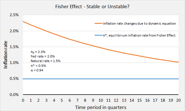
In this graph, the autoregressive coefficient is 0.94 (less than 1.0). Consequently, we can see that through time, inflation (orange line) is trending toward the Fisher equilibrium inflation rate of 0.5% (blue line). In this case, the Fisher Effect is stable.
Unstable Fisher Effect
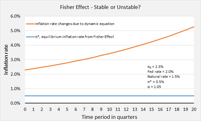
When α is greater than 1 we have an inflation rate that explodes upward or downward over time disrespecting the Fisher Effect. (Note: If inflation starts below π*, then inflation will fall instead of rise according to the equation.) Inflation in this case responds to other factors that override the Fisher Effect. In the following graph, the estimated α, autoregressive coefficient, is 1.05.
We can see how inflation keeps rising in spite of the Fisher Effect. In this case, the Fisher Effect is unstable.
One could imagine that the autoregressive coefficient was very high during the Weimar Republic in Germany just after World War I. Even though the nominal interest stayed steady between 3% and 5%, inflation sky-rocketed. There were strong inflationary pressures that overcame the Fisher Effect, such as rebuilding the country to printing money to pay off foreign debt.
So, Is the Current Fisher Effect Stable or Unstable?
Drum roll please… This is the finale.
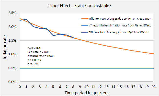
Now that we have our model, how does current data match up to it? Inflation data (CPI less food & energy) is added to the model for 1st quarter 2012 until 1st quarter 2014.
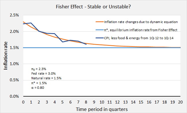
Inflation is trending fairly well along the path of a stable Fisher Effect. This is evidence that the Fisher Effect is working. Inflation is trending lower so as to raise the real rate (currently -1.2%) to its natural rate of 1.5%. But where exactly will the lower inflation rate become stable? Let’s now raise the Fed rate to a projected 3.0% from the 2.0% in the model. The equilibrium inflation rate that satisfies the Fisher Effect will now rise from 0.5% to 1.5% (light blue line rises). The autoregressive coefficient is changed to 0.80 to match the inflation data with a dynamic path.
Even in this case, inflation is following the path of a stable Fisher Effect, but it is not clear how low inflation is trending. Is it trending to 1.5% or lower? The answer depends on the projected steady-state of the Fed rate.
Conclusion
The Fisher Effect wants inflation to align itself with a steady nominal Fed rate and the natural real rate of interest. Eventually the Fed rate will rise to a long run steady-state around 2.0% according to the Federal Reserve. Thus, the Fed rate will stay low and steady for some years to come. Assuming that the natural real rate is 1.5%, inflation would then keep falling to below 1.0% according to a stable Fisher Effect.
The Fisher Effect currently depends upon weak inflationary pressures. If there were strong inflationary pressures from aggressive fiscal policy or a rising labor share, inflation could escape the Fisher Effect and rise upward instead of fall. There is caution against that type of instability. There are measures to moderate inflation as the Fed’s reserves are bloated. It would be safer to keep the autoregressive coefficient below 1.0.
For the moment, inflation is falling along the dynamic path toward a lower inflation rate. So I conclude that α, the autoregressive coefficient, must be below 1.0.
Assuming from the above evidence that the Fisher Effect is active and stable, inflation will go lower the longer the Fed’s nominal rate stays near the zero lower bound. If the Fed were to raise the Fed rate, inflation would not fall as much. A higher Fed rate would lead to a higher Fisher equilibrium inflation rate. Theoretically, inflation would stop falling.
The Fed rate should have started rising over a year ago. Low inflation is a big concern. However, raising the Fed rate now is a complicated issue. There would be adverse effects globally. There are economically sensitive reasons to keep the Fed rate low. They don’t call it the liquidity “trap” for nothing.


